Probabilistic Machine Learning
GPstuff - birthdates demo
Birthdates demo using Gaussian Processes, demo_births
Demonstration of analysis of birthday frequencies in USA 1969-1988 using Gaussian process with several components. Demonstration includes two parts a) analysis of data having sum of births for each day of year and b) analysis for whole time series. Data source: National Vital Statistics System natality data, as provided by Google BigQuery and exported to cvs by Chris Mulligan (sum data http://chmullig.com/wp-content/uploads/2012/06/births.csv) and Robert Kern (whole time series http://www.mechanicalkern.com/static/birthdates-1968-1988.csv)
Pieces of code
Part A) analysis of data having sum of births for each day of year
Get data and preprocess:
% load data
d=dataset('File','births.csv','Delimiter',',');
% remove strange values
d(d.births<1e3,:)=[];
% multiply leap day value by 4
d.births(60)=d.births(60)*4;

% target and covariate
y=d.births;
n=numel(y);
x=[1:n]';
% normalize
[xn,xmean,xstd]=normdata(x,mean(x),1);
[yn,ymean,ystd]=normdata(y);
The model is constructed as follows:
% priors
pl = prior_logunif();
pn = prior_logunif();

% smooth non-periodic component
gpcf1 = gpcf_sexp('lengthScale', 10, 'magnSigma2', 1);
% periodic component
gpcfp = gpcf_periodic('lengthScale', 2, 'magnSigma2', .05, ...
                      'period', 7,'lengthScale_sexp', 20, 'decay', 1, ...
                      'lengthScale_prior', pl, 'magnSigma2_prior', pl, ...
                      'lengthScale_sexp_prior', pl);

% Student's t model
lik = lik_t('sigma2', 0.05, 'sigma2_prior', pn, 'nu', 2);
% Student's t model with unknwon nu
% this is little slower to optimise as nu goes below 2 and EP uses more time
%lik = lik_t('sigma2', 0.05, 'sigma2_prior', pn, 'nu', 2, 'nu_prior', pn);

% construct the model
gp = gp_set('lik', lik, 'cf', {gpcf1, gpcfp},'latent_method','EP','jitterSigma2',1e-5);
Optimize hyperparameters to maximum a posteriori estimates
% optimise the hyperparameters (MAP)
opt=optimset('TolFun',1e-3,'TolX',1e-5,'Display','iter');
gp=gp_optim(gp,xn,yn,'opt',opt);
Make predictions to training set and also compute leave-one-out cross-validation estimates
% Predictions and training log predictive density
[Eft, Varft, lpyt] = gp_pred(gp, xn, yn);sum(lpyt)
% Leave-one-out cross-validation
[Efl, Varfl, lpyl] = gp_loopred(gp, xn, yn);sum(lpyl)
Do predictions also with different covariance functions
% Predictions for different components
Eft1 = gp_pred(gp, xn, yn, 'predcf', 1);
Eft2 = gp_pred(gp, xn, yn, 'predcf', 2);
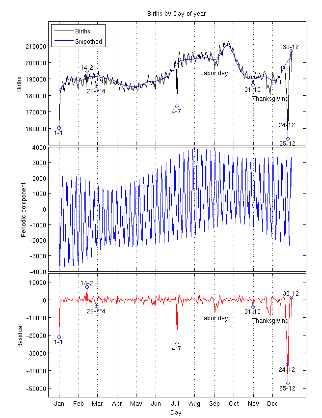
Plot results for the first part
% plot
figure
set(gcf,'units','centimeters');
set(gcf,'pos',[35 2 18.5 24]);
set(gcf,'papertype','a4','paperorientation','portrait',...
'paperunits','centimeters','paperposition',[ 0 0 21.0 29.7]);
clf
% get tight_subplot from
% http://www.mathworks.com/matlabcentral/fileexchange/27991
ha = tight_subplot(3, 1, .005, [.05 .05], [.15 .05]);
axes(ha(1))
Eft1n=denormdata(Eft1,ymean,ystd);
plot(x,y,'k',x,Eft1n,'b')
set(gca,'ytick',[160000:10000:210000],'yticklabel',[160000:10000:210000],'ylim',[150000 225000])
set(gca,'xtick',1+cumsum([0 31 29 31 30 31 30 31 31 30 31 30]),'xticklabel',[],'xgrid','on','xlim', [-16 388])
legend('Births','Smoothed',2)
specdays=[1 1;2 14;2 29;7 4;10 31;12 24;12 25;12 30];
for i1=1:size(specdays,1)
  sdi(i1)=find(d.month==specdays(i1,1)&d.day==specdays(i1,2));
end
sds=[-1 1 -1 -1 -1 -1 -1 1];
for i1=1:size(specdays,1)
  line(sdi(i1),y(sdi(i1)),'marker','o')
  if i1==3
    h=text(sdi(i1),y(sdi(i1)),sprintf('%d-%d*4', specdays(i1,2), specdays(i1,1)));
  else
    h=text(sdi(i1),y(sdi(i1)),sprintf('%d-%d', specdays(i1,2), specdays(i1,1)));
  end
  set(h,'HorizontalAlignment','center');
  if sds(i1)>0
    set(h,'VerticalAlignment','bottom')
  else
    set(h,'VerticalAlignment','top')
  end
end
ldi=find(d.month==9&d.day==1)
h=text(ldi,y(ldi)-5000,'Labor day');
set(h,'VerticalAlignment','bottom')
set(h,'HorizontalAlignment','center');
ldi=find(d.month==11&d.day==28)
h=text(ldi,y(ldi)-8000,'Thanksgiving');
set(h,'VerticalAlignment','bottom')
set(h,'HorizontalAlignment','center');
title('Births by Day of year')
ylabel('Births')
axes(ha(2))
plot(x,denormdata(Eft2,0,ystd),'b')
ylabel('Periodic component')
set(gca,'xtick',1+cumsum([0 31 29 31 30 31 30 31 31 30 31 30]),'xticklabel',[],'xgrid','on','xlim', [-16 388])
ylabel('Periodic component')
axes(ha(3))
r=y-denormdata(Eft,ymean,ystd);
plot(x,r,'r')
ylim([-50000 10000])
set(gca,'ytick',[-50000:10000:10000],'yticklabel',[-50000:10000:10000],'ylim',[-55000 15000])
set(gca,'xtick',1+cumsum([0 31 29 31 30 31 30 31 31 30 31 30]),'xticklabel',{'Jan' 'Feb' 'Mar' 'Apr' 'May' 'Jun' 'Jul' 'Aug' 'Sep' 'Oct' 'Nov' 'Dec'},'xgrid','on','xlim', [-16 388])
ylabel('Residual')
specdays=[1 1;2 14;2 29;7 4;10 31;12 24;12 25;12 30];
for i1=1:size(specdays,1)
  sdi(i1)=find(d.month==specdays(i1,1)&d.day==specdays(i1,2));
end
sds=[-1 1 -1 -1 -1 -1 -1 1];
for i1=1:size(specdays,1)
  line(sdi(i1),r(sdi(i1)),'marker','o')
  if i1==3
    h=text(sdi(i1),r(sdi(i1)),sprintf('%d-%d*4', specdays(i1,2), specdays(i1,1)));
  else
    h=text(sdi(i1),r(sdi(i1)),sprintf('%d-%d', specdays(i1,2), specdays(i1,1)));
  end
  set(h,'HorizontalAlignment','center');
  if sds(i1)>0
    set(h,'VerticalAlignment','bottom')
  else
    set(h,'VerticalAlignment','top')
  end
end
ldi=find(d.month==9&d.day==1)
h=text(ldi,r(ldi)-5000,'Labor day');
set(h,'VerticalAlignment','bottom')
set(h,'HorizontalAlignment','center');
ldi=find(d.month==11&d.day==28)
h=text(ldi,r(ldi)-8000,'Thanksgiving');
set(h,'VerticalAlignment','bottom')
set(h,'HorizontalAlignment','center');
xlabel('Day')
Part B) analysis of data having sum of births for each day of year
Get data and preprocess:
% load data
d=dataset('File','birthdates-1968-1988.csv','Delimiter',',');
y=d.births;
% fixed special days in USA
specdays=[1 1;1 2;2 1 4;2 29;4 1;7 4;7 5;10 31;12 22;12 23;12 24;12 25;12 26;12 27;12 28;12 29;12 30;12 31];
% construct additional covariates for fixed special days
xs=zeros(n,size(specdays,1));
xsw=zeros(n,size(specdays,1));
for i1=1:size(specdays,1)
  xs(:,i1)=double(d.month==specdays(i1,1)&d.day==specdays(i1,2));
  xsw(:,i1)=double(d.month==specdays(i1,1)&d.day==specdays(i1,2)&d.day_of_week>=6);
end
% construct additional covariates for floating special days
uyear=unique(d.year);
n=numel(y);
xss=zeros(n,2);
% Labor day
for i1=1:numel(uyear)
  q=find(d.year==uyear(i1)&d.month==9&d.day_of_week==1);
  xss(q(1),1)=1;
  xss(q(1)+1,1)=1;
end
% Thanksgiving
for i1=1:numel(uyear)
  q=find(d.year==uyear(i1)&d.month==11&d.day_of_week==4);
  xss(q(4),2)=1;
  xss(q(4)+1,2)=1;
end
% Memorial day
for i1=1:numel(uyear)
  q=find(d.year==uyear(i1)&d.month==5&d.day_of_week==1);
  xss(q(end),3)=1;
end
% combine covariates
x=[[1:n]' xs xsw xss];
m=size(x,2)
% normalize
xn=x;
[yn,ymean,ystd]=normdata(y);
Construct the model and optimize:
% priors
pl = prior_logunif();
pn = prior_logunif();

% smooth non-periodic component
gpcf1 = gpcf_sexp('lengthScale', 365, 'magnSigma2', .7, 'selectedVariables', 1);
% faster changing non-periodic component
gpcf2 = gpcf_sexp('lengthScale', 10, 'magnSigma2', .4, 'selectedVariables', 1);
% periodic component with 7 day period
gpcfp1 = gpcf_periodic('lengthScale', 2, 'magnSigma2', .1, ...
                      'period', 7,'lengthScale_sexp', 20, 'decay', 1, ...
                      'lengthScale_prior', pl, 'magnSigma2_prior', pl, ...
                      'lengthScale_sexp_prior', pl, 'selectedVariables', 1);
% periodic component with 365.25 day period
gpcfp2 = gpcf_periodic('lengthScale', 100, 'magnSigma2', .1, ...
                      'period', 365.25,'lengthScale_sexp', 1000, 'decay', 1, ...
                      'lengthScale_prior', pl, 'magnSigma2_prior', pl, ...
                      'lengthScale_sexp_prior', pl, 'selectedVariables', 1);
% linear component for special days
gpcfl=gpcf_linear('coeffSigma2',1,'selectedVariables',2:m);

% Gaussian model
lik = lik_gaussian('sigma2', 0.1, 'sigma2_prior', pn);

% construct the model
gp = gp_set('lik', lik, 'cf', {gpcf1, gpcf2, gpcfp1, gpcfp2, gpcfl})

% optimise the hyperparameters (MAP)
opt=optimset('TolFun',1e-3,'TolX',1e-4,'Display','iter','DerivativeCheck','off');
gp=gp_optim(gp,xn,yn,'opt',opt);
Do predictions and compute leave-one-out cross-validation estimates
% Predictions and training log predictive density
[Eft, Varft, lpyt] = gp_pred(gp, xn, yn);sum(lpyt)
% Leave-one-out cross-validation
[Efl, Varfl, lpyl] = gp_loopred(gp, xn, yn);sum(lpyl)

% Predictions for different components
[Eft1, Varft1] = gp_pred(gp, xn, yn, 'predcf', 1);
[Eft2, Varft2] = gp_pred(gp, xn, yn, 'predcf', 2);
[Eft3, Varft3] = gp_pred(gp, xn, yn, 'predcf', 3);
[Eft4, Varft4] = gp_pred(gp, xn, yn, 'predcf', 4);
[Eft5, Varft5] = gp_pred(gp, xn, yn, 'predcf', 5);
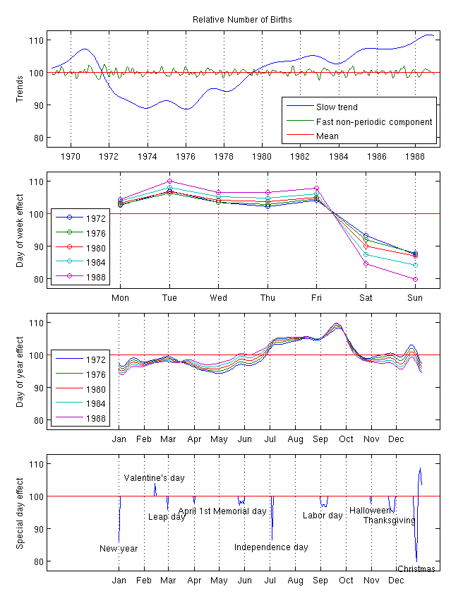
Plot results
figure
set(gcf,'units','centimeters');
set(gcf,'pos',[35 2 18.5 24]);
set(gcf,'papertype','a4','paperorientation','portrait',...
'paperunits','centimeters','paperposition',[ 0 0 21.0 29.7]);
clf
% get tight_subplot from
% http://www.mathworks.com/matlabcentral/fileexchange/27991
ha = tight_subplot(4, 1, .04, [.05 .05], [.1 .05])

% reshape 7 day periodic component
ywft3s=reshape(Eft3(1:7301),7,1043)';
ywft3s=ywft3s(:,[6:7 1:5]);
% trend is not completely seprated to the first smooth component so
% compute the trend in the 7 day periodic component
trend3=interp1(3:7:7303,mean(ywft3s'),1:n)';

axes(ha(1))
% Eft1+trend3 = smooth trend from component 1 plus trend from the
%               7 day periodic component
% Eft2 = faster changing non-periodic component
plot(x(:,1),denormdata(Eft1+trend3,ymean,ystd)/ymean*100,x(:,1),denormdata(Eft2,ymean,ystd)/ymean*100)
set(gca,'xtick',1+cumsum([0+365 365+365 366+365 365+365 366+365 365+365 366+365 365+365 366+365 365+365]),'xticklabel',1970:2:1988,'xgrid','on','xlim',[-100 7405])
ylim([77 113])
line(xlim,[100 100],'color', 'r')
legend('Slow trend','Fast non-periodic component','Mean',4)
ylabel('Trends')
title('Relative Number of Births')

% compute index for start of each year
ywys=reshape(d.year(1:7301),7,1043)';
ywys=ywys(:,[6:7 1:5]);
Y=1969:1988;
for i1=1:numel(Y);
  qi(i1)=find(ywys(:,1)==Y(i1),1);
end

% detrend the first periodic component (note that this trend was
% added to smooth trend above)
ywft3s=denormdata(ywft3s,ymean,ystd)/ymean*100;
mywft3s=mean(ywft3s,2);
ywft3s=bsxfun(@minus,ywft3s,mywft3s)+100;

axes(ha(2))
% ywft3s = 7 day periodic component at different years
plot(ywft3s(qi(4:4:end),:)','-o')
set(gca,'xtick',1:7,'xticklabel',{'Mon' 'Tue' 'Wed' 'Thu' 'Fri' 'Sat' 'Sun'},'xgrid','on')
xlim([-.5 7.5])
ylim([77 113])
line(xlim,[100 100],'color', 'r')
legend('1972','1976','1980','1984','1988',3)
ylabel('Day of week effect')

% reshape 365.25 day periodic component
Y=1969:1988;
yyft4s=NaN+zeros(20,366);
for i1=1:numel(Y);
  for i2=1:366
    q=Eft4(d.year==Y(i1)&d.day_of_year==i2);
    if ~isempty(q)
      yyft4s(i1,i2)=q;
    end
  end
end
yyft4s=denormdata(yyft4s,ymean,ystd)/ymean*100;

axes(ha(3))
% yyft4s = 365.25 day periodic component at different years
plot(yyft4s(4:4:end,:)','-')
set(gca,'xtick',1+cumsum([0 31 29 31 30 31 30 31 31 30 31 30]),'xticklabel',{'Jan' 'Feb' 'Mar' 'Apr' 'May' 'Jun' 'Jul' 'Aug' 'Sep' 'Oct' 'Nov' 'Dec'},'xgrid','on','xlim', [-86 388])
line(xlim,[100 100],'color', 'r')
ylim([77 113])
legend('1972','1976','1980','1984','1988',3)
ylabel('Day of year effect')

% reshape special day component
for i1=1:366
  yft5(i1,1)=mean(Eft5(d.day_of_year==i1));
end

axes(ha(4))
% yft5 = special day effect
plot(denormdata(yft5,ymean,ystd)/ymean*100,'-')
set(gca,'xtick',1+cumsum([0 31 29 31 30 31 30 31 31 30 31 30]),'xticklabel',{'Jan' 'Feb' 'Mar' 'Apr' 'May' 'Jun' 'Jul' 'Aug' 'Sep' 'Oct' 'Nov' 'Dec'},'xgrid','on','xlim', [-86 388])
line(xlim,[100 100],'color', 'r')
ylabel('Special day effect')
ylim([77 113])
yft5d=denormdata(yft5,ymean,ystd)/ymean*100;
h=text(1,yft5d(1),'New year','HorizontalAlignment','center','VerticalAlignment','top');
h=text(45,yft5d(45),'Valentine''s day','HorizontalAlignment','center','VerticalAlignment','bottom');
h=text(60,yft5d(60),'Leap day','HorizontalAlignment','center','VerticalAlignment','top');
h=text(92,yft5d(92),'April 1st','HorizontalAlignment','center','VerticalAlignment','top');
h=text(148,yft5d(148)-1,'Memorial day','HorizontalAlignment','center','VerticalAlignment','top');
h=text(186,yft5d(186),'Independence day','HorizontalAlignment','center','VerticalAlignment','top');
h=text(248,yft5d(248)-1,'Labor day','HorizontalAlignment','center','VerticalAlignment','top');
h=text(305,yft5d(305),'Halloween','HorizontalAlignment','center','VerticalAlignment','top');
h=text(328,yft5d(328)-1.5,'Thanksgiving','HorizontalAlignment','center','VerticalAlignment','top');
h=text(360,yft5d(360),'Christmas','HorizontalAlignment','center','VerticalAlignment','top');