
Probabilistic Machine Learning
GPstuff - classification demo
2-class Classification problem, 'demo_classific1'
In this demonstration program a Gaussian process is used for 2 class classification problem. The inference is conducted via Laplace, EP and MCMC
The demonstration program is based on synthetic two class data used by B. D. Ripley (http://www.stats.ox.ac.uk/pub/PRNN/). The data consists of 2-dimensional vectors that are divided into two classes, labeled -1 and 1. Each class has a bimodal distribution generated from equal mixtures of Gaussian distributions with identical covariance matrices.
There are two data sets from which other is used for training and the other for testing the prediction. The trained Gaussian process misclassifies the test data only in ~10% of cases. The decision line and the training data is shown in the figure below.
The code of demonstration program (without plotting commands) is shown below.
% Training data
S = which('demo_classific');
L = strrep(S,'demo_classific.m','demos/synth.tr');
x=load(L);
y=x(:,end);
y = 2.*y-1;
x(:,end)=[];
[n, nin] = size(x);

% Test data
xt1=repmat(linspace(min(x(:,1)),max(x(:,1)),20)',1,20);
xt2=repmat(linspace(min(x(:,2)),max(x(:,2)),20)',1,20)';
xt=[xt1(:) xt2(:)];

% Create covariance functions
gpcf1 = gpcf_sexp('lengthScale', [0.9 0.9], 'magnSigma2', 10);

% Set the prior for the parameters of covariance functions
pl = prior_unif();
pm = prior_sqrtunif();
gpcf1 = gpcf_sexp(gpcf1, 'lengthScale_prior', pl,'magnSigma2_prior', pm); %

% Create the GP structure (type is by default FULL)
gp = gp_set('cf', gpcf1, 'lik', lik_probit(), 'jitterSigma2', 1e-9);
%gp = gp_set('cf', gpcf1, 'lik', lik_logit(), 'jitterSigma2', 1e-9);

% ------- Laplace approximation --------
% Set the approximate inference method
% (Laplace is default, so this could be skipped)
gp = gp_set(gp, 'latent_method', 'Laplace');

% Set the options for the scaled conjugate optimization
opt=optimset('TolFun',1e-3,'TolX',1e-3,'MaxIter',20,'Display','iter');
% Optimize with the scaled conjugate gradient method
gp=gp_optim(gp,x,y,'optimf',@fminscg,'opt',opt);

% Make predictions
[Ef_la, Varf_la, Ey_la, Vary_la, Py_la] = gp_pred(gp, x, y, xt, 'yt', ones(size(xt,1),1) );


% ------- Expectation propagation --------
% Set the approximate inference method
gp = gp_set(gp, 'latent_method', 'EP');

% Set the options for the scaled conjugate optimization
opt=optimset('TolFun',1e-3,'TolX',1e-3,'Display','iter');
% Optimize with the scaled conjugate gradient method
gp=gp_optim(gp,x,y,'optimf',@fminscg,'opt',opt);

% Make predictions
[Ef_ep, Varf_ep, Ey_ep, Vary_ep, Py_ep] = gp_pred(gp, x, y, xt, 'yt', ones(size(xt,1),1) );


% ------- MCMC ---------------
% Set the approximate inference method
% Note that MCMC for latent values requires often more jitter
gp = gp_set(gp, 'latent_method', 'MCMC', 'jitterSigma2', 1e-6);

% Sample using default method, that is, surrogate and elliptical slice samplers
% these samplers are quite robust with default options
[gp_rec,g,opt]=gp_mc(gp, x, y, 'nsamples', 220);
% Remove burn-in
gp_rec=thin(gp_rec,21,2);

% Make predictions
[Ef_mc, Varf_mc, lpy_mc, Ey_mc, Vary_mc] = ...
    gp_pred(gp_rec, x, y, xt, 'yt', ones(size(xt,1),1) );
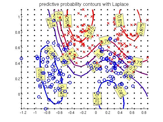
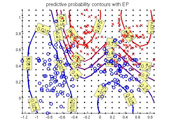
Figure 1. The training points and decision line.