Logistic GP for density estimation and regression demo

Demonstration of fast logistic GP for density estimation and regression. The inference method is described in

• Jaakko Riihimäki and Aki Vehtari (2014). Laplace approximation for logistic Gaussian process density estimation and regression. Bayesian analysis, in press. Online 3 February, 2014.

1D density estimation

The figure below shows the 1D density estimation of the classical Log-acidity data and the Galaxy data. The figure is the same as in Andrew Gelman, John B. Carlin, Hal S. Stern, David B. Dunson, Aki Vehtari and Donald B. Rubin (2013). Bayesian Data Analysis, Third Edition. Chapman and Hall/CRC.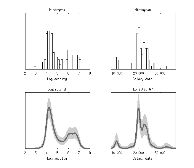

Code for the 1D density estimation example

S = which('demo_lgpdens');
L = strrep(S,'demo_lgpdens.m','demodata/log_acidity.txt');
x=load(L);
datarange=[2 8];
xt=linspace(datarange(1),datarange(2),400)';

subplot(2,2,1)
xth=linspace(datarange(1),datarange(2),40)';
ph=hist(x,xth);ph=ph./sum(ph)./diff(xth(1:2));
h=bar(xth,ph,1,'w');
set(gca,'ytick',[])
xlim(datarange)
ylim([0 1])
box on
xlabel('Log acidity')
title('Histogram')

subplot(2,2,3)
lgpdens(x,xt,'gpcf',@gpcf_matern32);
box on
set(gca,'ytick',[])
xlabel('Log acidity')
title('Logistic GP')

S = which('demo_lgpdens');
L = strrep(S,'demo_lgpdens.m','demodata/galaxy.txt');
x=load(L);
datarange=[7000 37000];
xt=linspace(datarange(1),datarange(2),200)';

subplot(2,2,2)
xth=linspace(datarange(1),datarange(2),40)';
ph=hist(x,xth);ph=ph./sum(ph)./diff(xth(1:2))
h=bar(xth,ph,1,'w');
xlim(datarange)
set(gca,'ytick',[],'xtick',[1e4 2e4 3e4],...
  'xticklabel',{'10 000' '20 000' '30 000'})
ylim([0 3e-4])
box on
xlabel('Galaxy data')
title('Histogram')

subplot(2,2,4)
lgpdens(x,xt,'gpcf',@gpcf_matern32);
title('Logistic GP')
xlabel('Galaxy data')
ylim([0 3e-4])
box on
set(gca,'ytick',[],'xtick',[1e4 2e4 3e4],...
  'xticklabel',{'10 000' '20 000' '30 000'})

2D density estimation

The figure below shows the 2D density estimation of the classical Old-faithful data and a simulated Banana data.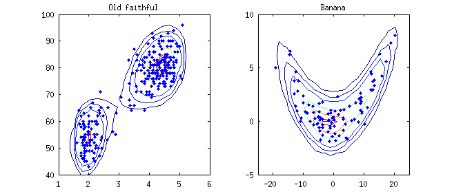

Code for the 2D density estimation example

% Old faithful
subplot(1,2,1)
S = which('demo_lgpdens');
L = strrep(S,'demo_lgpdens.m','demodata/faithful.txt');
x=load(L);
lgpdens(x,'range',[1 6 40 100]);
line(x(:,1),x(:,2),'LineStyle','none','Marker','.')
title('Old faithful')

% Banana-shaped
subplot(1,2,2)
n=100;
setrandstream(0,'mrg32k3a');
b=0.02;x=randn(n,2);
x(:,1)=x(:,1)*10;x(:,2)=x(:,2)+b*x(:,1).^2-10*b;
lgpdens(x,'range',[-30 30 -5 20],'gridn',26);
line(x(:,1),x(:,2),'LineStyle','none','Marker','.')
axis([-25 25 -5 10])
title('Banana')

Density regression

The figure below shows the density regression of the classical Rats data. Usually this data is modelled using linear model, but it is easy to that the groeth speed is declining in time.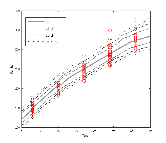

Code for the density regression example

S = which('demo_lgpdens');
L = strrep(S,'demo_lgpdens.m','demodata/rats');
load(L);
xx=repmat(x,30,1);
xx=xx(:);
yy=yy(:);
lgpdens([xx yy],'range',[5 40 100 400],'cond_dens','on');
hold on
plot(x,y,'ro')
xlabel('Time')
ylabel('Weight')
box on