Probabilistic Machine Learning
GPstuff - monotonic GP demo
Monotonic GP demo, demo_monotonic2
Demonstration of benefit of monotonicity information in GP modeling. GPstuff implements monotonicity using virtual derivative observations and expectation propagation method as described in
- Riihimäki and Vehtari (2010). Gaussian processes with monotonicity information. Journal of Machine Learning Research: Workshop and Conference Proceedings, 9:645-652. Online
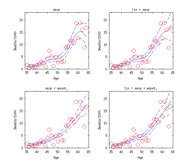
Monotonicity in prediction of mortality given age
The first example (demo_monotonic.m) uses mortality data from Broffitt, J. D. (1988). Increasing and increasing convex Bayesian graduation. Transactions of the Society of Actuaries, 40(1), 115-48.
The figure below displays the predictions with models with and without the monotonicity constraint. The monotonicity constraint allows inclusion of sensible prior information that death rate increases as age increases. The effect is shown most clearly for larger ages where there is less observations, but also overall reduction in uncertainty related to the latent function can be seen.
Code for the mortality example
S = which('demo_monotonic2');
L = strrep(S,'demo_monotonic2.m','demodata/broffit.txt');
d=readtable(L,'Delimiter',';');
x=d.age;
y=d.y;
z=d.N.*(sum(d.y)./sum(d.N));
zt=repmat(1000,size(y)).*(sum(d.y)./sum(d.N));
[xn,nd.xmean,nd.xstd]=normdata(x);

% Basic GP
pl=prior_t();
pm=prior_sqrtt();
cfl=gpcf_linear('coeffSigma2',10^2,'coeffSigma2_prior',[]);
cfs=gpcf_sexp('lengthScale',.4,'lengthScale_prior',pl,'magnSigma2_prior', pm);
lik=lik_poisson();
% Alternative GP models a) sexp b) lin + sexp
gpa = gp_set('lik', lik, 'cf', {cfs}, 'jitterSigma2', 1e-6, 'latent_method', 'EP');
gpb = gp_set('lik', lik, 'cf', {cfl cfs}, 'jitterSigma2', 1e-6, 'latent_method', 'EP');

% 1) sexp
subplot(2,2,1)
gpiaa=gp_ia(gpa,xn,y,'z',z);
gp_plot(gpiaa,xn,y,'z',z,'zt',zt,'target','mu','normdata',nd)
hold on
plot(d.age,d.y./d.N*1000,'ro')
axis([34 65 0 23])
xlabel('Age')
ylabel('Deaths/1000')
title('sexp')

% 2) sexp + monotonicity
subplot(2,2,3)
opt=optimset('TolX',1e-1,'TolFun',1e-1,'Display','iter');
gpam=gpa;gpam.xv=xn(2:2:end);
gpam=gp_monotonic(gpam,xn,y,'z',z,'nvd', 1, 'optimize', 'on', ...
                  'opt', opt, 'optimf', @fminlbfgs);
gpiaam=gp_ia(gpam,xn,y,'z',z);
gp_plot(gpiaam,xn,y,'z',z,'zt',zt,'target','mu','normdata',nd)
hold on
plot(d.age,d.y./d.N*1000,'ro')
axis([34 65 0 23])
xlabel('Age')
ylabel('Deaths/1000')
title('sexp + monot.')

% 3) lin + sexp
subplot(2,2,2)
gpiab=gp_ia(gpb,xn,y,'z',z);
gp_plot(gpiab,xn,y,'z',z,'zt',zt,'target','mu','normdata',nd)
hold on
plot(d.age,d.y./d.N*1000,'ro')
axis([34 65 0 23])
xlabel('Age')
ylabel('Deaths/1000')
title('lin + sexp')

% 4) lin + sexp + monotonicity
subplot(2,2,4)
opt=optimset('TolX',1e-1,'TolFun',1e-1,'Display','iter');
gpbm=gpa;gpbm.xv=xn(2:2:end);
gpbm=gp_monotonic(gpb,xn,y,'z',z,'nvd', 1, 'optimize', 'on', ...
                  'opt', opt, 'optimf', @fminlbfgs);
gpiabm=gp_ia(gpbm,xn,y,'z',z);
gp_plot(gpiabm,xn,y,'z',z,'zt',zt,'target','mu','normdata',nd)
hold on
plot(d.age,d.y./d.N*1000,'ro')
axis([34 65 0 23])
xlabel('Age')
ylabel('Deaths/1000')
title('lin + sexp + monot.')
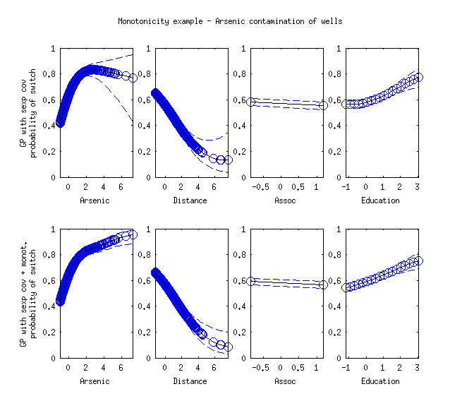
Monotonicity in predicting probability of well switching
Another example (not included in GPstuff distribution) is the prediction of the probability that user of an arsenic contaminated well switches to a safe well in Bangladesh rural area. Data has been analysed, e.g, in the book Data Analysis Using Regression and Multilevel/Hierarchical Models by Gelman and Hill (2007).
The figure below show the predictions with models with and without monotonicity constraint. The monotonicity constraint allows inclusion of sensible prior information that probability of switching increases if the arsenic concentration or education increases or the distance to the nearest safe well decreases.