Gaussian Process regression demo, demo_regression1

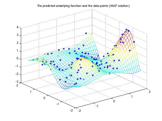
The demonstration program solves a simple 2-dimensional regression problem using Gaussian process. The data in the demonstration has been used in the work by Christopher J. Paciorek and Mark J. Schervish (2004). The training data has an unknown Gaussian noise and can be seen in Figure 1. We conduct the inference with Gaussian process using squared exponential covariance function.

Description

The regression problem consist of a data with two input variables and one output variable with Gaussian noise. The observations y are assumed to satisfy

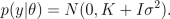
and f is an underlying function, which we are interested in. We place a zero mean Gaussian process prior for f, which implies that at the observed input locations latent values have prior

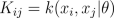
where K is the covariance matrix, whose elements are given as

Since both likelihood and prior are Gaussian, we obtain a Gaussian marginal likelihood

By placing a hyperprior for hyperparameters, p(th), we can find the maximum a posterior (MAP) estimate for them by maximizing

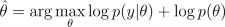
If we want to find an approximation for the posterior of the hyperparameters, we can sample them using Markov chain Monte Carlo (MCMC) methods.

After finding MAP estimate or posterior samples of hyperparameters, we can use them to make predictions for f:

Pieces of code

The model is constructed as follows:

% Create likelihood
lik = lik_gaussian('sigma2', 0.2^2);

% Create covariance function
gpcf = gpcf_sexp('lengthScale', [1.1 1.2], 'magnSigma2', 0.2^2)

% Set some priors
pn = prior_logunif();
lik = lik_gaussian(lik,'sigma2_prior', pn);
pl = prior_unif();
pm = prior_sqrtunif();
gpcf = gpcf_sexp(gpcf, 'lengthScale_prior', pl, 'magnSigma2_prior', pm);

% Create GP
gp = gp_set('lik', lik, 'cf', gpcf);
	      

We will make the inference first by finding a maximum a posterior estimate for the hyperparameters via gradient based optimization. After this we will use grid integration and Markov chain Monte Carlo sampling to integrate over the hyperparameters.

% Set the options for the scaled conjugate optimization
opt=optimset('TolFun',1e-3,'TolX',1e-3,'Display','iter');
% Optimize with the scaled conjugate gradient method
gp=gp_optim(gp,x,y,'optimf',@fminscg,'opt',opt);
	      

Make predictions of the underlying function on a dense grid and plot it. Below Eft_map is the predictive mean and Varf_map the predictive variance.

[xt1,xt2]=meshgrid(-1.8:0.1:1.8,-1.8:0.1:1.8);
xt=[xt1(:) xt2(:)];
[Eft_map, Varft_map] = gp_pred(gp, x, y, xt);
	      

We can also integrate over the hyperparameters. Following line performs grid integration and makes predictions for xt

[gp_array, P_TH, th, Eft_ia, Varft_ia, fx_ia, x_ia] = gp_ia(gp, x, y, xt, 'int_method', 'grid');

Alternatively we can use MCMC to sample the hyperparameters. (see gp_mc for details) The hyperparameters are sampled using default method, that is, slice sampling.

% Do the sampling (this takes approximately 5-10 minutes)
% 'rfull'   will contain a record structure with all the sampls
% 'g'       will contain a GP structure at the current state of the sampler
[gp_rec,g,opt] = gp_mc(gp, x, y, 'nsamples', 220);

% After sampling we delete the burn-in and thin the sample chain
gp_rec = thin(gp_rec, 21, 2);

% Make the predictions
[Eft_mc, Varft_mc] = gp_pred(gp_rec, x, y, xt);