Probabilistic Machine Learning
GPstuff - disease mapping demo
Disease mapping problem demonstration, 'demo_spatial1'
Description
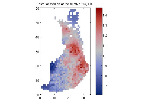
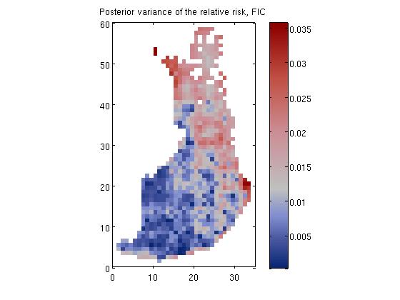
The model constructed is as follows. The number of death cases Y_i in area i is assumed to satisfy
where E_i is the expected number of deaths (see manual for explanation on how E_i is evaluated) at area i and r_i is the relative risk.
We place a zero mean Gaussian process prior for log(R), R = [r_1, r_2,...,r_n], which implies that at the observed input locations latent values, f, have prior
where K is the covariance matrix, whose elements are given as

We place a hyperprior for hyperparameters, p(theta)
Pieces of code
The data are in the following parameters:
- xx = co-ordinates
- yy = number of deaths
- ye = the expexted number of deaths
We construct the model. Below we constuct Mátern nu=3/2 covariance function and Poisson likelihood. We set Student-t priors for the covariance function parameters (length-scale and magnitude). Then we initialize GP model structure with FIC sparse approximation (the inducing inputs are set with set_PIC function). For the last we define that the latent variables are marginalized out with Laplace approximation.
S = which('demo_spatial1');
data = load(strrep(S,'demo_spatial1.m','demos/spatial1.txt'));

x = data(:,1:2);
ye = data(:,3);
y = data(:,4);

% Now we have loaded the following parameters
% x = co-ordinates
% y = number of deaths
% ye = the expected number of deaths

[n,nin] = size(x);

% Create the covariance functions
gpcf1 = gpcf_matern32('lengthScale', 5, 'magnSigma2', 0.05);
pl = prior_t('s2',10);
pm = prior_sqrtunif();
gpcf1 = gpcf_matern32(gpcf1, 'lengthScale_prior', pl, 'magnSigma2_prior', pm);

% Create the likelihood structure
lik = lik_poisson();

% Create the FIC GP structure so that inducing inputs are not optimized
gp = gp_set('type', 'FIC', 'lik', lik, 'cf', {gpcf1}, 'X_u', Xu, ...
'jitterSigma2', 1e-4, 'infer_params', 'covariance');

% --- MAP estimate with Laplace approximation ---

% Set the approximate inference method to Laplace approximation
gp = gp_set(gp, 'latent_method', 'Laplace');

% Set the options for the scaled conjugate optimization
opt=optimset('TolFun',1e-3,'TolX',1e-3,'Display','iter');
% Optimize with the scaled conjugate gradient method
gp=gp_optim(gp,x,y,'z',ye,'opt',opt);

% make prediction to the data points
[Ef, Varf] = gp_pred(gp, x, y, x, 'z', ye, 'tstind', [1:n]);

% --- IA ---
[gp_array,pth,th,Ef,Varf] = gp_ia(gp, x, y, x, 'z', ye, ...
   'int_method', 'grid', 'step_size',2);

% --- MCMC ---

% Set the approximate inference method to MCMC
gp = gp_set(gp, 'latent_method', 'MCMC', 'latent_opt', struct('method',@scaled_hmc));

% Set the sampling options

% HMC-param
hmc_opt.steps=3;
hmc_opt.stepadj=0.01;
hmc_opt.nsamples=1;
hmc_opt.persistence=0;
hmc_opt.decay=0.8;

% HMC-latent
latent_opt.nsamples=1;
latent_opt.nomit=0;
latent_opt.persistence=0;
latent_opt.repeat=20;
latent_opt.steps=20;
latent_opt.stepadj=0.15;
latent_opt.window=5;

% Here we make an initialization with
% initial sampling parameters
[rgp,gp,opt]=gp_mc(gp, x, y, 'z', ye, 'hmc_opt', hmc_opt, 'latent_opt', latent_opt);

% Now we reset the sampling parameters to
% achieve faster sampling
opt.latent_opt.repeat=1;
opt.latent_opt.steps=7;
opt.latent_opt.window=1;
opt.latent_opt.stepadj=0.15;
opt.hmc_opt.persistence=0;
opt.hmc_opt.stepadj=0.03;
opt.hmc_opt.steps=2;

opt.display = 1;
opt.hmc_opt.display = 0;
opt.latent_opt.display=0;

% Define help parameters for plotting
xii=sub2ind([60 35],x(:,2),x(:,1));
[X1,X2]=meshgrid(1:35,1:60);

% Conduct the actual sampling.
% Inside the loop we sample one sample from the latent values and
% parameters at each iteration. After that we plot the samples so
% that we can visually inspect the progress of sampling
while length(rgp.edata)<1000
[rgp,gp,opt]=gp_mc(gp, x, y, 'record', rgp, 'z', ye, opt);
% ...plotting code not shown
end