Stochastic volatility GP demo, demo_stochasticvolatility

Demonstration of stochastic volatility modeling using a GP with an input dependent noise model. Inference is made using Laplace approximation and EP. EP inference is described in

• Ville Tolvanen, Pasi Jylänki and Aki Vehtari (2014). Expectation propagation for nonstationary heteroscedastic Gaussian process regression. In Machine Learning for Signal Processing (MLSP), 2014 IEEE International Workshop on, DOI:10.1109/MLSP.2014.6958906. Online.

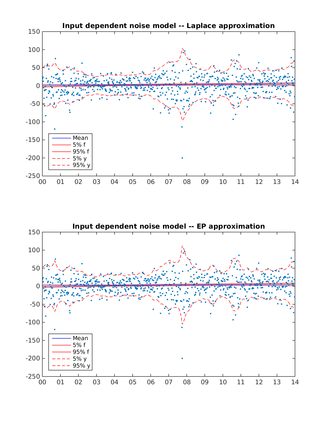
Stochastic volatility model for S&P 500 stock index weekly closing value 2001-2014

Data is change in S&P 500 stock index weekly closing value from 2001-01-02 to 2014-12-29.

The figure below displays the predictions with Laplace approximation and Expectation Propagation (EP). The model is able to capture the changes in the volatility using either inference approach.

Code for the stochastic volatility (input dependent noise) example

%% Data
% Stochastic volatility model for change in
% S&P 500 stock index weekly closing value from 2001-01-02 to 2014-12-29
S = which('demo_stochasticvolatility');
L = strrep(S,'demo_stochasticvolatility.m','demodata/sp500_weekly.csv');
d=dataset('File',L,'Delimiter',',');
d.Datenum=datenum(d.Date);
% order from oldest to newest
x=flipud(d.Datenum);
x=x(2:end)-x(1);
% normalise
[xn,nd.xmean,nd.xstd]=normdata(x);
% order from oldest to newest
y=flipud(d.Close);
% change in closing price
y=diff(y);
% normalise
[yn,nd.ymean,nd.ystd]=normdata(y);
%
n=numel(y);

%% Covariance functions
pl = prior_t('s2',1);
pm = prior_t('s2',1); 
gpcf1 = gpcf_sexp('lengthScale', 1, 'magnSigma2', 0.5, ...
                  'lengthScale_prior', pl, 'magnSigma2_prior', pm);
gpcf2 = gpcf_exp('lengthScale', 1, 'magnSigma2', 0.1, ...
                 'lengthScale_prior', pl, 'magnSigma2_prior', pm);

%% Inference using Laplace approximate

% Create the likelihood structure. Don't set prior for sigma2 if covariance
% function magnitude for noise process has a prior.
lik = lik_inputdependentnoise('sigma2', 0.1, 'sigma2_prior', prior_fixed());

% NOTE! if multiple covariance functions per latent is used, define
% gp.comp_cf as follows:
% gp = gp_set(..., 'comp_cf' {[1 2] [5 6]};
gp = gp_set('lik', lik, 'cf', {gpcf1 gpcf2}, 'jitterSigma2', 1e-9, 'comp_cf', {[1] [2]});

% Set the approximate inference method to Laplace
gp = gp_set(gp, 'latent_method', 'Laplace');
% For more complex problems, maxiter in latent_opt should be increased.
% gp.latent_opt.maxiter=1e6;

% Set the options for the optimization
opt=optimset('TolFun',1e-3,'TolX',1e-3,'Derivativecheck','off','Display','iter');
% Optimize with the scaled conjugate gradient method
gp=gp_optim(gp,xn,yn,'opt',opt);

% make prediction to the data points
[Ef, Varf,lpyt, Ey, Vary] = gp_pred(gp, xn, yn);
Ef11=Ef(1:n);Ef12=Ef(n+1:end);
Varf11=diag(Varf(1:n,1:n));
prctmus=[Ef11-1.645*sqrt(Varf11) Ef11 Ef11+1.645*sqrt(Varf11)].*nd.ystd+nd.ymean;
prctys=[Ey-1.645*sqrt(Vary) Ey Ey+1.645*sqrt(Vary)].*nd.ystd+nd.ymean;

figure;
a4
% plot mean and 5% and 95% quantiles
subplot(2,1,1)
plot(x,prctmus(:,2),'b',x,prctmus(:,1),'r',x,prctmus(:,3),'r',x,prctys(:,1),'r--',x,prctys(:,3),'r--',x,y,'.')
datetick('x',11)
title('Input dependent noise model -- Laplace approximation');
legend('Mean','5% f','95% f','5% y','95% y','location','southwest')


%% Inference using EP

% note that lik_epgaussian could be used to include input dependent
% magnitude, too, see demo_epinf
sigma2=1;
lik = lik_epgaussian('sigma2', sigma2, 'sigma2_prior', prior_fixed(), ...
                     'int_likparam', true, 'inputparam', true);

% Set latent options
latent_opt = struct('maxiter',1000, 'df',0.8, 'df2',0.6, 'tol',1e-6, ...
                    'parallel', 'on', 'init_prev','off', 'display','off');

% NOTE! if multiple covariance functions per latent is used, define
% gp.comp_cf as follows:
% gp = gp_set(..., 'comp_cf' {[1 2] [5 6]};
gp2 = gp_set('lik', lik, 'cf', {gpcf1 gpcf2}, ...
             'jitterSigma2', 1e-9, 'comp_cf', {1 2}, ...
             'latent_method', 'EP', 'latent_opt', latent_opt);

gp2 = gp_optim(gp2,xn,yn,'opt',opt, 'optimf', @fminscg);
[Ef, Varf, lpyt, Ey, Vary] = gp_pred(gp2, xn, yn);
prctmus=[Ef(:,1)-1.645*sqrt(Varf(:,1)) ...
         Ef(:,1) ...
         Ef(:,1)+1.645*sqrt(Varf(:,1))].*nd.ystd+nd.ymean;
prctys=[Ey(:,1)-1.645*sqrt(Vary(:,1)) ...
         Ey(:,1) ...
         Ey(:,1)+1.645*sqrt(Vary(:,1))].*nd.ystd+nd.ymean;

subplot(2,1,2)
plot(x,prctmus(:,2),'b',x,prctmus(:,1),'r',x,prctmus(:,3),'r',x,prctys(:,1),'r--',x,prctys(:,3),'r--',x,y,'.')
datetick('x',11)
title('Input dependent noise model -- EP approximation');
legend('Mean','5% f','95% f','5% y','95% y','location','southwest')