
Probabilistic Machine Learning
GPstuff - classification demo
Survival analysis using accelerated failure time GP model demo
This example is from
- Andrew Gelman, John B. Carlin, Hal S. Stern, David B. Dunson, Aki Vehtari and Donald B. Rubin (2013). Bayesian Data Analysis, Third Edition. Chapman and Hall/CRC.
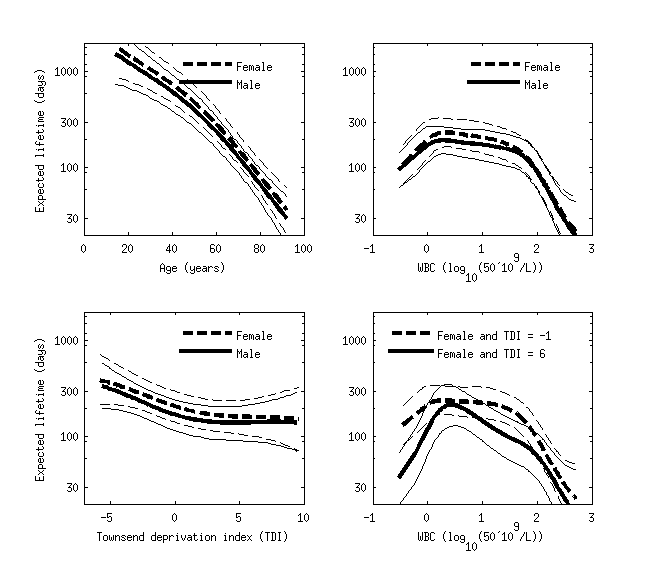
Example data set is leukemia survival data in Northwest England presented in (Henderson, R., Shimakura, S., and Gorst, D. (2002). Modeling spatial variation in leukemia survival data. Journal of the American Statistical Association, 97:965-972).
The latent inference is made using Laplace approximation and covariance function and likelihood parameter inference is made using CCD integration.
Figure below shows estimated conditional comparison of each predictor with all others fixed to their mean values or defined values. The model has found clear nonlinear patterns, and the right bottom subplot also shows that the conditional comparison associated with WBC has an interaction with the Townsend deprivation index. The benefit of the Gaussian process model was that we did not need to explicitly define any parametric form for the functions or define any interaction terms.
Code for the demo
See demo_survival_aft.m for the additional plotting code.
% First load data
S = which('demo_survival_aft');
L = strrep(S,'demo_survival_aft.m','demodata/leukemia.txt');
leukemiadata=load(L);

% leukemiadata consists of:
% 'time', 'cens', 'xcoord', 'ycoord', 'age', 'sex', 'wbc', 'tpi', 'district'

% survival times
y0=leukemiadata(:,1);
y=y0;
% scale survival times (so that constant term for the latent function can be small)
y=y0/geomean(y0);

ye=1-leukemiadata(:,2); % event indicator, ye = 0 for uncensored event
                        %                  ye = 1 for right censored event

% for simplicity choose 'age', 'sex', 'wbc', and 'tpi' covariates
x0=leukemiadata(:,5:8);
x=x0;
[n, m]=size(x);
% transform white blood cell count (wbc), which has highly skewed
% distribution with zeros for measurements below measurement accuracy
x(:,3)=log10(x(:,3)+0.3);
% normalize continuous covariates
[x(:,[1 3:4]),xmean(:,[1 3:4]),xstd(:,[1 3:4])]=normdata(x(:,[1 3:4]));
% binary sex covariate is not transformed
xmean(2)=0;xstd(2)=1;

% Create the covariance functions
cfc = gpcf_constant('constSigma2_prior',prior_sinvchi2('s2',1^2,'nu',1));
cfl = gpcf_linear('coeffSigma2',1,'coeffSigma2_prior',prior_sinvchi2('s2',1^2,'nu',1));
cfs = gpcf_sexp('lengthScale', ones(1,m),'lengthScale_prior',prior_t('s2',1^2,'nu',1),'magnSigma2_prior',prior_sinvchi2('s2',1^2,'nu',1));

% Create the likelihood structure
% log-logistic works best for this data
lik = lik_loglogistic();
%lik = lik_loggaussian();
%lik = lik_weibull();

% Create the GP structure
gp = gp_set('lik', lik, 'cf', {cfc cfl cfs}, 'jitterSigma2', 1e-8);
% classically used linear model could be defined like this
%gp = gp_set('lik', lik, 'cf', {cfc cfl}, 'jitterSigma2', 1e-8);

% Set the approximate inference method to Laplace
% Laplace is default, so this line could be skipped
gp = gp_set(gp, 'latent_method', 'Laplace');
%gp = gp_set(gp, 'latent_method', 'EP');

% Set the options for the optimization
opt=optimset('TolFun',1e-3,'TolX',1e-3,'Display','iter');
% Optimize with the BFGS quasi-Newton method
gp=gp_optim(gp,x,y,'z',ye,'opt',opt,'optimf',@fminlbfgs);
% CCD integration over parameters
gpia=gp_ia(gp,x,y,'z',ye,'opt_optim',opt,'optimf',[]);
% Leave-one-out cross-validation
[~,~,lploo]=gp_loopred(gpia,x,y,'z',ye);sum(lploo)
% -1629 for linear + squared exponential
% -1662 for linear only